Closing short near the Money Call to Reduce Gamma Risk on EEM Diagonal Spread

EEM has been performing OK relative to the general market last week. My EEM diagonal call spread was working fine. The short June 9 $42 call option that was sold 3 weeks ago for $0.27 was approaching its expiration date with 3 days left from Tuesday, June 6. It was near the money as EEM price was around $41.72 and Delta was around 0.46. The position had relatively high Gamma risk which could turn the short call into a significant loss in a couple of days even though the EEM price just increased a little bit to above $42. Therefore, I bought back the short call for $0.10 to eliminate Gamma risk and to lock in a profit of $0.17 on the short call on Tuesday, as I twitted in my StockTwits message.

After that, I have EEM long call January 19, 2018 $38 naked. Since it seemed to form a small ascending triangle pattern with MACD turning up and travelling in the upper trending channel as shown in the chart below, I did not sell another short call. I’ll short new calls when the stock movement provides the signal to sell.

 

The option’s Gamma risk could have a big impact on option strategies that include short options when the expiration date is coming closer. This is because option Gamma increases dramatically as the option approaches expiration, particularly for options At-The-Money (ATM). Therefore, many option strategies that sells options for protection and/or for benefit of time decay need to watch for Gamma risks as the expiration comes closer. This and the definition of option Gamma are very well explained in the article on Understanding Gamma by Dough.com. I also had a study on the option Greeks in my previous post: A Summary of Effects of Prices, Time, Volatility on Option Greeks.

The diagonal spread involves short options and therefore need to take Gamma risk into account in its option adjustment rules. There are two major impacts on diagonal spreads due to the characteristic of option Gamma. We already discussed the first impact near the expiration. This results one short option closing rule that it should be closed in the last week when the stock price is close to the option’s strike price.

The second Gamma impact on the diagonal spread is the possibility of Delta inversion. Since the option closer to expiration has higher Gamma than that of the option that is far from expiration, the Delta changes faster for the option closer to expiration as well.

Thus, the short option in a diagonal spread which is closer to the expiration may have its Delta changing quicker than that of the long option which is farther away from expiration. When the short option’s Delta exceeds the long option’s Delta, it’s called a Delta Inversion. The wider the expiration dates of the short and long options, the more frequently it’s likely to happen.

Delta inversion causes originally bullish diagonal call spreads to lose money if the stock prices continue to go up as expected. It also causes originally bearish diagonal put spreads to lose money if the stock continues to fall.

For example, a short call option may have a Delta of 0.50 while the long call option may have a Delta of 0.70. As the short option gets closer to expiration and near-the-money, its Gamma increases faster. If stock price increases $1, the Delta of the short call option may increase faster to 0.75 while the Delta of the long call option may increase slower to 0.72. So, the composite Delta of the diagonal call spread changes from +0.20 (bullish) to -0.03 (0.72-0.75, bearish). The originally bullish call diagonal spread starts to lose money if the stock prices increase as the trader expects in the beginning of the diagonal trade.

Therefore, diagonal spread management rules are required to avoid the Delta inversion in order to trade the strategy profitably. What I’ve leant is that the short option should be rolled when the composite Delta of a diagonal spread gets closer to 0.15 area, or the short option’s Delta get above 0.60. If we roll up or roll out the short call that is likely to cause Delta inversion, the composite Delta gets expanded wider to have more profit room for stock price increases. If the stock prices reverse direction from here, we can keep selling new options as well.

How many premiums are fair for short options?

As an option seller, I've been interested to know if the premiums I received for selling options are fair or not. However, there are so many factors that impact the premiums of sold options. To obtain a reasonable feeling of the fairness, I studied the TLT option spreads that I dealt with in the last few months. I used TLT short options of similar probability of success, same amount of capital requirement with the same width ($5) for the vertical spreads, and day to expiration around 56+/-7 days. In this way, I was able to reduce the number of variables for this comparison.

My goal is to receive 10% to 13% return on capital (premium$/width$5) for all ETF's that I trade. For the TLT options that meet my criteria, it means the premium should be above $0.50. Based on the above table, it looks to me the following conclusions are true for the options of similar probability and risks.

• Put premiums are higher than call premiums under similar conditions
• Premiums are higher when the short option bid and ask prices are narrower
• Premiums are higher when open interests are larger
• Premiums are higher when Delta differences between short and long strikes are larger
• Premiums are higher when the IV differences (Skew) between short and long strikes are smaller
• Premiums may not be higher with longer DTE in the analyzed range
• Higher IV of the option does not guarantee higher premium

My biggest surprise is that the higher IV's do not always provide higher premium or ROC. In October  turbulent trading, I could obtain higher ROC as IV was much higher in those days. But now, the IV of TLT is still high and yet its option premiums offer less ROC. I found other more liquid options (i.e. IWM) offer reasonable ROC (>10%) at the same time. The only reason I could find so far was the lack of open interests in the options. So I would conclude the lack of option liquidity means lower ROC for option sellers and the middle option price of bid and ask may not be fair.

In general, I believe this is one way for option sellers to estimate the fairness of option premiums as they use options of similar parameters for the comparison.

Time decay chart and analysis of individual put options

As planned analysis of my closed naked put selling of FXI & TBT, I updated my ThinkScript to chart the delta-adjusted time value decay of Out-of-The-Money (OTM) put options. The updated script uses an average moving line to show the actual time decay of the option under analysis. Additionally, it shows the Bollinger bands of the time value in order to illustrate the overall time decay effect. BB showed a big contraction in the last 2 weeks in both cases. Some people may say the Bollinger band of the time decay is a wavy cone as a result.

To me, it suggests the option can be bought back 2 weeks prior to expiration. The charts provides supportive evidence to the conceptual drawing of OTM time decay after the inflection point in my previous post.

For the FXI put option trade, it demonstrated a more volatile time decay curve as the price of FXI fluctuated around the sold option strike. It can be found that time value was relatively high when the option is ATM.

For the TBT put trade, the price of TBT stayed OTM all the time. So the the time value at the last 4 weeks was quite small. When did time value start quick decline? It was difficult to tell from the chart. In June to July time frame, the option time value had big decline as a result of the rapid price ascend, even though we are using Delta-adjusted time value on the chart. In August to October time frame, the stock price dropped but the option price also fell as a result of time decay.

In the next posts, I'll examine the option time decay from a return of capital perspective.

The time decay chart of a put option adjusted by Delta

Time decay is a fascinating part of option premium selling strategy. In my quest searching for suitable time decay, I'd like to get clear picture in areas such as what are good entry and exit points that capture rapid option time decay in a option's life span. I had posted a conceptual OTM option time decay chart  and an actual OTM time decay chart before. This time, I further studied the time decay of my naked FXI put option sold 3 weeks ago with the help of ThinkScript.

Since option price changes with underlying stock due to the impact of Delta, I decided to observe the option premium decay after taking out the Delta-induced option price changes. The option time value in my study was restricted to changes due to volatility (Vega) and Theta mainly in this way:
Option time value = extrinsic value  =
previous price + Delta-induced change + sum of Vega and Theta induced changes.

Using a simple approximation of Delta-induced option price changes, I was able to chart the Delta-adjusted time decay curve of the naked put which took out the Delta-induced change in the above equation. The directional price change from Delta is calculated as shown below using ThinkScript:
plot TmValExclDelta = extrVal - ((absValue(Delta()) + gamma() * opChange)/2) * (opChange);

The entire script is downloadable for anyone who is interested. It can be used as a base for other option premium analysis. The resulted chart is downloadable in a PDF file if anyone needs to see a clearer picture.

As shown in the above chart, I found a few key points below. I think a picture is worthless a thousand words. There are other points that can be observed from it as well. Note the left vertical axis is FXI ETF price and right vertical axis is FXI Dec$37.5 put option price.

• The FXI option price was high while its time value was low as FXI dropped below the strike price.
• The FXI option time decay acceleration started at about 2.5 months before expiration.
• The naked put sold at Delta around 0.3 and its time decay stayed close to the bottom downtrending line as FXI price consolidated for 3 weeks.

One of the interesting point to me is that this option started rapid decay around 2.5 months. If one sells the option on 2.5 months before expiration and exit it at around 1 month before expiration, he would capture a good amount of premium values with relatively smooth time decay as well. 

OTM Option Time Decay and its Exit Time

TastyTrade posted a video on Theta Based Exits for Sold Options on Youtube. It was quite educational. I’d like to share with everyone some of my review and thoughts on this topic.

On the time decay part, we sell options of delta of 0.30 to 0.35, which implies the ITM probability around 30% to 35% by expiration date. A credit is received after the option selling, which is similar to selling insurance premium. The OTM option time decay manner is somewhat different from that of ATM options which is show-cased in a lot of option text books. Based on the video introduction, the OTM option with Delta around 0.33 has a time decay chart as shown below. [Note I believe the hosts made a minor error in describing the units of the axes. The horizontal axis represent the passing time of the option in weeks (not days as they said) for an option that expires in 10 weeks. The vertical axis is the   option price x 100 in Dollars (not option price as they mentioned).]

For OTM options, the option’s price is the same as its extrinsic value. Time decay functions similar to insurance premium. This chart suggests OTM option (Delta = 0.33) price decay is relatively faster at around the first 7 weeks (49 days), which is the inflection point. After that, the time decay slows down as the price of the option has already dropped significantly and there is not much value left. The big assumption is that the OTM option stays OTM, although it was not elaborated how much price movement of the underlying could have to maintain such as time decay pattern. The discussion seemed to suggest that this 0.30 ~ 0.35 Delta OTM time decay chart is the merge of a 0.4 ~ 0.6 Delta ATM option at the 1^st few weeks and a 0.1 ~ 0.2 Delta OTM option at the last few weeks.

In reality, it may be difficult to come up with the above curve for any specific options, as prices always fluctuate. Demonstrating the daily rate of return on capital (ROC) in a chart is also interesting and it can give very good clues on when to exit this type of trades. Thus, this is one area that I intend to investigate in the future with the help of ThinkScript.

On the management of winners using Theta decay for exits, I believe it’s a great rule and Tom has been telling many of his students for a long time. Once most of the premium is decayed through time, the remaining value is quite small and the rate of decay becomes very slow. From risk to reward perspective, it will not look good if we try to gain a small reward that remains in the last couple of weeks before expiration. Therefore, it makes sense to buy back the sold option in the last couple of weeks immediately after the inflection point, as the return of capital gets smaller.

TOS offers free trades for option buy-backs within a nickel. However, many options at the inflection points are likely to be worth above $0.05. Only very low priced options can meet the free commission trade criteria. It would be much helpful for retail traders if TOS could offer free buy back trades at the inflection points such as Delta <= 0.10 or price <=  $0.10 J

Where should be a good point of entry to sell the options? This is not discussed in this video. But from the chart, it appears to tell us that 8 to 7 weeks before expiration is a good entry point where the option starts to accelerate its time decay. This entry point coincides with the option selling days used by Supertrade Karen.

In summary, the video discussed option premium selling by exploring the relationship of statistical probability (success rate and occurrence rate), return on capital, and management of winners. It did not use the option Greeks that much. Even though Theta had been mentioned in the whole discussion, the value of Theta or the trend of Theta was not shown at all.

The so called “Theta based exit” should be more accurately named as “Time decay based exit” in my opinion as Theta is only one component of the time decay. The other components for time decay include implied volatility/Vega and Delta which also change with time. There is no guarantee that Theta provides the most time decay when compared to Vega and Delta.

A review on trading option Greeks

A few years ago, I attended a couple of Dan Passarelli's live Webinars and remembered him as one of the most knowledgeable and passionate option trading educators. Recently, I bought his book "Trading Options Greeks: How Time, Volatility, and Other Pricing Factors Drive Profits (Bloomberg Financial)". I did spend sometime reading interesting sections of the book. So I created an initial post on the summary table of the effects of prices, time and volatility on option Greeks and another study on the implied volatility and its time decay. Since this book is pretty useful for me, I'd like to share some thoughts on it with my readers.

Compared with a couple of other option trading books I have that cover similar topics, this book describes a mathematically simple way to manually calculate approximate option price changes using the option Greeks. It is a unique part of this book that it uses many examples to illustrate how to estimate option price changes using the option Greeks with approximation equations that involve a few addition, subtraction, multiplication and division only.

I consider this book an intermediate level one for option traders that require a solid understanding of the Greeks, as this book goes a little further beyond the introduction phase. It explains what the Greeks are, and more importantly, how the Greeks change under various scenarios which is missing in most other option trading books. This book also gives introductions about various option spread strategies and volatility spreads in particular.

I don't consider it as advanced level, as it rarely describes Greeks and their changes at option portfolio level or for complex option positions. It's not an option trading system book as well, since it does not offer any specific criteria for trade entry, exit or adjustment. To get more detailed descriptions about the 5-star user rated book (as of today) and other reader comments, you can click on the book image below.

The Grand Summary of Effects of Prices, Time, Volatility on Option Greeks - Part 1

I had thought I had necessary understanding of the effects of stock prices, strike prices, time to expiration and implied volatility on option Greeks. But after some more study, I realized that I need to know more details about their effects on major option Greeks such as Delta, Gamma, Vega and Theta. Today, I had some time to finish the 1st part of my study and posted here to share with everyone who may be interested. I have  not seen this kind of table in any option materials yet. Hopefully, it will be helpful for the people trading options on the Greeks.

As you can see, I'll need to complete the other cases where stock price and volatility go down. After that, I'll review my past posts related to option Greeks and make sure they are consistent with this table.

Update: The Gamma changes against time elapse need further review. It's common knowledge as expiration gets closer, Gamma risk become larger. Thus, the ATM strike Gamma must be increasing a lot faster than the OTM Gamma decreases. Also it's possible that really far OTM Gamma decreases while closer OTM Gamma may not decrease. In this way, an OTM portfolio will have Gamma increases over time.

The subject of option Greek changes against time, price and volatility for a premium selling portfolio requires a series of studies in the future and I'll post it as I progress.

Another study of option implied volatility and its time decay

After my recent discovery of the volatility discrepancy in TOS analyzer, I started investigating the IV of options. In one of my post, I have showed a chart illustrating the time decay of Vega. This weekend, I further studied the time decay of implied volatility and would like to note down and share with readers.

Implied volatility is always associated with a time frame. For the composite IV of options (IV of all option chains and expiration , the time frame is 1 year of trading days. It's annualized. To estimate the IV of an individual option which has a definite life time, we can calculate the daily IV first, then multiply it by the remaining trading days to derive the actual IV of the specific option.

The daily IV = Annualized IV / square root of 256 trading days = IV / 16 in brief.

Therefore, the IV of an individual option = daily IV x square root of trading days to expiration.

Based on the above approximation, it's easy to understand that as days pass by, the IV of each option gets smaller and smaller.

Also note that the individual option's IV is directly proportional to the square root of trading days. At intraday time frame of trading, market makers will adjust the IV continuously. If other influencing factors do not change, the option's IV will decrease from market open to close. This is the intraday time decay, specially big for weekends as noted for option Theta before. In fact, Vega has very similar characteristics as Theta with the exception that IV can change in two directions (up and down) and time can only elapse.

We often use $VIX (CBOE volatility index) as a measure of overall market IV. It's actually derived as the IV of a hypothetical 30-day option of SPX using a weigthed average of two nearest expiration series. The time frame associated with VIX is 30 days here. For option trades that use two month back options, the volatility could be square root (2x22) x IV/square root(22) = 1.41 x IV which is significant bigger.

Unfortunately, TOS does not offer the feature to display IV decay over time for individual options at the moment.

The actual time decay Chart of OTM option Theta and Vega

I'm interested to understand the real time-decay of my high probability option selling monthly income portfolio. I tried to use the TOS software without success, since it's designed to show the Greeks of various strike prices mainly. The ThinkScript has some bugs that prevent me from writing a script to display the time decay for every trading day. If ThinkOrSwim can fix the bugs, I may be able to design such a script for TOS chart.

For now, it's possible to display Theta and Vega hourly chart for a single option. So I used a sold SPX May put as the initial example which is shown below. The TOS chart also has a bug that prevent me to display it in daily chart. I had to use intraday (4 hour is selected to present more data) chart for this purpose.

As we can see from the chart, the sold put kept losing value as time passed by and SPX rose. It's apparent that Vega kept losing value as time passed by. It also reacted inversely to the SPX price (in the same direction as IV). My goal is to display implied volatility and Vega's impact on option values. Unfortunately, the IV functionality in ThinkScript is not working. I'm waiting for a response from TOS tech support to see if they are going to fix these type of issues.

The Theta time decay ((32.5-25)/32.5 = 23%) in last month was not that much when compared with that ((170-57)/170 = 66%) of the Vega. The Theta's reaction to SPX's price is similar as Vega: a reverse relationship with price (direct relationship with IV). Theta peaked on 2nd last Thursday as that was the lowest price day of SPX in the period. At the same day, the put option price also had a smaller peak to the market sell-off.

It looks to me an iron condor with negative Vega would benefit more time decay than a double calendar which has positive Vega if the spreads are opened two months before expiration. Is it really true? I'll have to analyze it in a future post.

What it really matters is that the put option price has been falling down since the open date. This is the ultimate effect of all Greeks. I'll continue to monitor the option price drop till the expiration day to get a overall picture of the option time decay.

Update: Since this post is becoming one of the popular ones of my blog, I'd like to update additional thoughts here.
1. As shown in the top section of the graph, it's apparent that Delta or index price changes have the most significant impact on option prices. The sold put option is out of the money, so the option price is made of time value solely. Using a moving average of the option price in the chart may better illustrate the decay of time value. I can do that in a future post.
2. Option Theta value becomes larger as the option price increases. But the percentage of Theta over time value may change different. I will create a ThinkScript to track the Theta value as a percentage of time value in a future study as well.

The issue of ThinkOrSwim software when analyzing volatility's impact caused by Vega

I have been using the TOS analyzer to estimate the volatility's impact on portfolio or position's profit/loss for quite some time. I believe there are many other option traders & instructors analyzing it in the same way as I did. Recently I discovered there was a major issue in my past volatility analysis using the TOS platform.

After identification of some discrepancies in volatility used in TOS in my first post of the series and another discussion on how to estimate option implied volatility changes of each position in a Beta-weighted portfolio, I'd like to discuss the real issue here and figure out a way to work around it.

The above chart of ThinkOrSwim showes that Delta and Gamma are Beta-weighted while the Theta and Vega are not. For Theta, there is no issue since each instrument contribute time decay daily based on its corresponding Theta. But for Vega, the situation is different from Theta and somewhat similar to Delta. Like P&L caused by Delta of each instrument, the P&L caused by Vega of each instrument changes differently in each market day.

For example, if SPX moves 1%, the VIX may change 2 points. The IV of OTM options of the SPX position may change 0.6 percentage point. At the same day, RUT may move 1.2% (just an example number) point and its volatility RVX may change 2.5 points. The IV of OTM options of the RUT position may change 0.8 percentage point. So if we assume a 0.6 point change of IV of the SPX beta weighted portfolio, and use the straight sum of the aggregated Vega to calculate the IV induced P&L, our results are not accurate at all. This is particularly an issue for larger trading capitals. The estimated results will be close to the actual P&L if we use some kind of special weights for Vega of each different position.

Besides the lack of proper weighting in the Vega analysis, I had used the analyzer by adjusting the volatility field according to VIX. I had assumed if SPX changes 10 points, the VIX is likely to change 1 point (which is OK). Then, I would adjust the volatility field by 1 point and observe the new P&L in the live price slice section. It usually generates a substantial change in P&L. This is a total overestimation of the volatility impact on P&L. In reality, the portfolio's IV does not change 1 point as the VIX does. The portfolio or position IV actually changes much less than the VIX, could be 30% of the VIX only.

In another word, if the IV of the position is adjusted for 1 point in the TOS analyzer, it would mean the VIX changes over 3 points and market has a major sell-off or jump-up. If we adjust the IV field by +2 points, it may require VIX to increase 6 points, which may correspond to SPX to drop 60 points.

I did not realized this before. So, it is an major error that I had in my previous Vega related calculations, including the post on proper Greek  values of Delta neutral portfolios.

The TOS analyzer does not help either. If a user increases the volatility field by 1, the analyzer increases all option IV by 1 and VIX (or RVX) by 1 as well. It gives user an impression that option IV changes at the same rate as the VIX. In the future, I need to figure out how to calculate the equivalent position IV change based on SPX changes so that we can use TOS analyzer more accurately.

Estimating option volatility changes using ThinkOrSwim Analyzer

Today, I'd to continue to discuss the TOS analyzer, option volatility, Vega and $VIX. This is the 2nd post on this topic after the post yesterday which focused a little bit more on the discrepancy side.

To have a good understanding of the impact of volatility on high probability option portfolio, I need to be able to estimate how the option portfolio P&L changes when volatility changes, using the TOS analyzer (or some other option analysis software in the future).  In particular, the values of volatility of each strike are different. So how do we estimate the portfolio P&L changes if we use one IV value in the TOS analyzer?

On 4-3, I recorded the following IV vs Strike chart during market hour. It revealed a couple of relationships that I could understand at the moment:

Volatility skews

• Put options have higher IV than call options
• Front month IV changes fastest and further back month IV changes slower
• Future month IV is visibly higher in the middle price range for put options only
• As strike prices increase, the IV of both call and put options decreases.

The IV of calls and puts in the chart appeared to increase 0.3 if SPX declined 10 points(which might cause VIX to drop 1 point). It is a significant observation for me that if VIX drops 1 point the IV's of my portfolio options may drop 0.3 only. I'll focus the overestimation of P&L changes from Vega x IV  in one of my future post.

I also captured the IV vs Strike chart today (11 days after the above one) during market hour. This time, I noticed the VIX & RVX had discrepancies in the quote pane and the Analyzer as shown in the circled fields. These numbers matched pretty well in my previous image. Now the IV appears to make slower changes with the SPX prices in the chart below as time passes by. In theory, the IV/Vega should keep decreasing to 0 at expiration day.

Option Volatility discrepancies in ThinkOrSwim Analyzer

Since my last post on option Theta time decay of my non-directional portfolio over weekend, I realized that there are some issues with the ThinkOrSwim options analyzer in the field of option implied volatility. Starting today, I'd like to describe them in a series of posts.

Right now, I'll discuss the discrepancy I found in a couple of charts around the April 1 time frame. I had recorded my portfolio's Greeks on 3-30 (Saturday) in the chart of my previous post, and on 4-1 morning session in the following chart.

Notably, the chart of 3-30 (which was a 3 day weekend for Wall Street) indicated the SPX volatility ($VIX)  of 13.26. This value was 0.56 higher than the close of last trading day on 3-28. So the ThinkOrSwim platform is tracking $VIX beyond the standard trading time. This extended hour value of VIX is incorporated  into the analyzer. Any customers using the analyzer at weekends for their portfolio analysis should be aware of this fact when working on volatility related analysis.

On 4-1, there was a significant SPX drop that caused $VIX to increase over $1.00 compared to the previous trading day. The TOS software had a VIX increase of 0.54 as shown in the table below.

	Pre Holiday	Sat	Mon	Wed	Wed-Sat
	28-Mar	30-Mar	1-Apr	3-Apr
SPX	1569	1569	1560	1559
DIFF		0	-9	-1	-10
VIX	12.7	13.26	13.8	13.43
DIFF		0.56	0.54	-0.37	0.17
Vola:$1595c	ThinkbackError	9.59	9.95	9.46
DIFF			0.36	-0.49	-0.13
Delta		-32.87	-27.37	-25.34
DIFF			5.5	2.03	7.53

Another important observation from the above table is that the IV of option strikes do not move in the same way as that of the VIX. However, the ThinkOrSwim analyzer uses VIX in the adjustment field of volatility.This can create some confusions when analyzing portfolio options. I'll write another post on this topic in the near future.

To track the option volatility on 3-28 for my analysis, I tried to use ThinkBack feature and found it does not provide the real history of Greeks since it gave a value over 10. It could not be the true value at the 3-30 market close since the real value on 3-30 (weekend) was 9.59. So people who use ThinkBack should be aware of this difference as well. I also tried ThinkOnDemand and found it does not offer info beyond a few strikes ATM.

Option Portfolio Theta time decay over weekends

Last Monday, my portfolio exhibited a relatively bigger profit change than what I expected as described in my previous post. It generated my interests in understanding how my portfolio P&L could change over weekends and holidays. After some studying, I'd like to summarize my initial findings here.

• At the portfolio level, the P&L changes with regard to SPX price changes may be larger if the non-SPX positions make bigger changes than normal (Beta), since the portfolio P&L used Beta-weighted Greeks. The Beta is an average calculated over a long time (1 year for TOS?)
• Weekend Theta decay starts around Friday, depending on the market condition at the time and on the market makers.
• Weekend Theta decay on Fridays does not show up in our Theta fields of the trading software, since our SW calculates Theta daily.
• Weekend Theta decay on Friday shows up in our option volatility reducing as the time value decreasing causes option price decreasing. This is the only way (?) we know if market markers have started weekend Theta time decay (if the true market IV does not change much).

To understand how the portfolio Theta changes with volatility, I used the TOS analyzer to see Theta increases as IV decreases as shown below. Beyond the BE zone, the Theta and IV relationship is probably meaningless since the option strikes are too far OTM to have meaningful Greeks.

Since Theta and IV move in the opposite direction, it would make sense for market makers to hold off the Theta time decay over the weekends that major events are expected to happen. In this way, market maker's manipulation of option prices is supported by both the Vega and Theta at the time of high volatility.

Reducing Feb portfolio delta

After yesterday's adjustment on SPX positions, the market continued to rise. Today, the portfolio had reached a Delta of -95. I considered it as too high for my portfolio. It had more than doubled the value of 36 for initial portfolio positions as I analyzed before, even though the current portfolio margin was about twice as the starting margin. So I reviewed existing positions and decided to close out the following IC which had its price close to the right drop-off point and a Delta of about 20.

After closing this IC with a minor profit, the overall portfolio still has a Delta of -75. The remaining Vega is about -325, equivalent to a Delta of 30 at the moment. Thus the effective Delta is around -45. I'll see how market does tomorrow to decide if any further action is required.

How SPX Vega changes with volatility and prices

I had studied how Vega (and other Greeks) changes with time in a previous post. Now I'd like to analyze how Vega changes with volatility and stock prices, since I'm using Vega to hedge the Delta in my monthly income portfolio selling high probability options, such as the Feb portfolio consisted of iron condors. With the help of TD Ameritrade's ThinkOrSwim analyzer, I captured the following image today to analyze my Vega changes with volatility and prices.

A picture is worth one thousand words. I have to digest this picture later when I have more time. For now, it looks to me the following is generally true in this picture. Note this is about the portfolio Vega, not the Vega of straight options.

• When IV increases 1%, 
•           Absolute(Vega) changes (decreases) about 7.5% at current price and VIX levels;
•           Absolute(Vega) changes (reduces) relatively larger at far far OTM strikes;
•           Vega changes little around break-even points;
• Vega is most negative at the center of the portfolio P&L chart.

The changes of portfolio Vega with volatility depend on price of the SPX as well. The absolute value of Vega is largest at the center of the P&L zone (Vega is largest ATM for straight options). For near the money strikes/zone, the abs(Vega ) decreases as volatility increases. This is similar to short options (short calls or puts) which profit when volatility decreases. If volatility increases, the short options lose value, meaning the Vega become smaller for the short option position.

The change of portfolio Vega described in this post also shows its conformance to the Vega changes of the straight options of calls and puts. For straight options, the Vega has the following characteristics in general.

• Vega vs time: Vega is higher when option has more time (shown in volatility skew of expiration cycles or Vega has time decay too!).
• Vega vs price: Vega (All Greeks except Delta) is highest for ATM options.
• Vega vs volatility: The higher the volatility, the higher the Vega? Not necessarily! 
• Vega is the option's sensitivity to its implied volatility and not directly proportional to volatility. Although the volatility values are higher for OTM put option strikes (shown in volatility skew of strikes), the option's sensitivities to IV for OTM options are lower, i.e. the Vega of OTM options is lower than that of the ATM options. However, for the same option strikes, Vega is higher if IV is higher.

Selling more premiums for Feb high probability portfolio

Market dropped in the last couple of days with higher volumes and the current intermediate uptrend is in danger. With volatility shooting up, I sold more premiums via February RUT and SPX iron condors with about 50 days to expiration.

Since market can drop rapidly and usually rise at a slower pace, I selected short strike prices in the following way: the short put strike had a delta around -20 as analyzed before and the short call strike had a delta around +24. This slight change in my strike selection rule is partially inspired by Karen's interview, and partially intended to reduce the effect of Vega of the high probability portfolio.

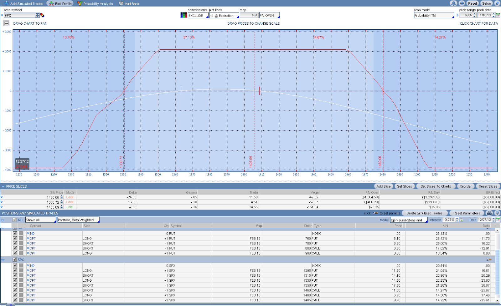
Using the above rule, I sold a RUT iron condor yesterday as shown in the graph below. IC's always have negative Vega, which favors reduction of volatility (market to rise). So the small negative delta of the position can neutralize the effect of Vega somewhat, making the position more market neutral.

Today, I also sold another SPX iron condor. My current portfolio has a Beta-weighted delta of -7, accommodating some down side market movements. The graph below recorded my current positions on RUT & SPX. I plan to complete my Feb portfolio tomorrow by adding another RUT time-decaying position.

To calculate how much Delta is needed to offset the Vega to obtain a market neutral portfolio, I used ATR to correlate Delta and Vega of SPX in the following way. Currently, SPX has ATR(30) of 14.3 and VIX has ATR(30) of 1.2. If the weighted SPX Delta x ATR is in the same range of VIX ATR x Vega, then the portfolio is about neutral. Thus, the Vega should be around 10 times of Delta to maintain the neutrality.

As an example, my Feb RUT IC has Vega of -47 and Delta of -5.3 is in the above range, making it perfectly market neutral. My 1st Feb SPX did not opened in this way while the 2nd SPX IC did. In the future, I will follow this rule when I intend to build market neutral portfolio in sideways market.

Analyzing short put delta of iron condor vs time decay

A few days back, I analyzed the relationship between OTM put Delta and Theta to understand how time decays for my short iron condors with different short put strikes.

I selected a short RUT put strike of Delta -0.22 in my 20 point wide put spread and another RUT short put strike of Delta -0.25. I kept the call spread within the iron condor the same in this analysis. The former (Delta = -0.22) had a slightly higher Theta (8.28) and Delta (-4.8) as shown in the graph below, while the Vega was similar (actually slightly higher as well) in both cases.

For the IC with short put of -0.25 Delta, it had a slightly lower Theta (7.95 vs 8.28) and Delta (-3.76 vs -4.8) while Vega remains close (-48.98 vs -49.28). The differently colored curves showed P&L of 6 calendar days apart. So the farther OTM IC would achieve a profit of $265 (vs $259 in closer OTM IC) near Jan expiration time if price does not change.

Overall, the analysis indicates time decays a little faster for the farther OTM option IC than the closer OTM option IC from 8 weeks to 4 weeks ahead of their expiration. Since I plan to exit positions 4 weeks before expiration whenever possible (as analyzed in a previous post), this farther OTM selection suits my strategy well and it provides higher probability as well. The cost of the change is less credit at the opening( but it does not cause slightly lower profit at the exit as one would expect).

How portfolio Greek changes within last 2 weeks of expiration

After a series of adjustments to my December high probability option trade portfolio, its P&L chart does not look really smooth anymore. The red expiration curve shows more profits if price goes higher by 10 or more SPX points while the portfolio delta is -26 which indicates more profits if price goes lower.  So I studied its Greeks verse time and prices using the ThinkOrSwim Analyzer.

First, let's take a look at how Delta changes as days get closer to expiration and prices fluctuates . After analyzing the delta changes in time, I found my delta would continue to go more negative in the next few days and it would start to increase only in the last 7 days to expiration as shown in the image below. The daily delta changes would be smaller if price increases to 1423 vicinity. I think it is most likely caused by the butterfly spreads that the portfolio has.

Secondly, let's review the daily changes of portfolio Theta. It's likely to change $10 to $20 each day next week at the current price range. However, if price goes a little over $10 which correlates to the top spot of the portfolio P&L curve, the Theta decay will be maximal for this portfolio. Theta decay will be smaller outside the indicated range in the following image.

Thirdly, the portfolio Vega is small (16) right now and it will double or triple in the next week even if price does not change. This is because the volatility will make up most of the time value in the last few days of expiration while Theta diminishes. The Vega will also shot up if price drop by 15 points.

Forth and lastly, let's see how profit and loss changes in the next 2 weeks. The following P&L chart shows profit will double 8 days later if price remain the same. If SPX price drops a bit, the profit will also increase. I believe the profit curve will have its top shifting to the 1430 area in the last 4 to 1 days of expiration to match the original expiration curve.

There are probably a number of conclusions that can be drawn from this type of Greek analysis and be incorporated in option trading rules. At the moment, I'm particularly interested in the daily Theta decay and Vega enrichment in the last 2 weeks before expiration. These two components are the time value of OTM options. For a market neutral portfolio comprising of many iron condors, the decrease of time values in the last 2 weeks will not be as dramatic as one would typically expect as long as the short strikes are still out-of-money.  It's an evidence supporting early IC exit (about 2+ weeks before expiration).  There is probably no significant loss of time decay if one starts IC 2 month ahead. Further study will be done to check it out.

Responded to Bull Attack at the High Probability Portfolio with Butterfly

On last Thursday, the 2 month out paper portfolio experienced a bull attack on the up side when the bulls reached the east boundary of the portfolio break-even points. The weaker RUT position suffered a small temporary blow as shown in the P&L chart below. Note the delta reached -52 with about 8 weeks to expiration. If the portfolio were built with shorter term options, it would cause lot more damages.

In response, I brought up a small, additional reserve capital to help fight the bulls by moving my eastern frontier further out, through a launch of a 2 month butterfly. The butterfly provides some longer term protection to my expiration territory and has little values of Greeks for the near term. The new battle map below indicates an approximate 10 point advance by my soldiers to the east boundary, with limited changes to the Greek values.

The portfolio is definitely stressed at the moment, as indicated by the Greeks. But my soldiers are still in good formation and they have plentiful of time waiting for the probabilistic market to assert himself. Of course, the portfolio is given a risk tolerance of $1,500 should SPX shots up $30 more points relentlessly to 1445 level, since high probability does not provide any guarantee for this specific trade. This is understood as the mind set of successful traders.

Note: There was cancellation trade for RUT Jan$830c. It resulted margin increase of $2000 and the new profit in the chart should be reduced by $870. I was busy testing different strikes and forgot to verify the existing strikes after I chose the final butterfly strikes.

Using P&L Curve and Greeks together to Manage Time-selling Portfolio

I have spent some time stream-lining my thoughts on managing the monthly income, time-selling and delta neutral portfolio with the Greeks and the Profit and Loss Graph. This is the last post on this topic for now.

The P & L Graph is a very good tool to present the current and expiration P & L across different prices. Its expiration (red) curve demonstrates the potential P & L during expiration. This is not easy to figure out from the Greeks if the expiration has many days to come.

The Greeks are good at estimating the immediate term (1 day or 2) P & L only, since they change significantly with prices and volatility. The Greeks are closely related to the current P & L (white) curve. For high priced stocks (i.e. SPX, RUT), it is not easy to estimate their P & L directly using the Greeks, because the stocks may change $10 a day but the Greeks (delta) measure the change of $1 only. A series of calculations would have to be made to get an approximate estimate of the portfolio P & L changes when using Greeks.

Combining the expiration P & L curve with Greeks should make it easier to manage the portfolio. At the option inventory building phase, I make every attempt to build a monthly portfolio with smooth expiration profit curve. As market attacks the portfolio with disruptive price changes, I will watch the market price against the expiration P & L. If the price is near the break even points, I would make adjustments. When making adjustment, I will manage the Greeks to neutralize market disruptions and try to maintain a smooth expiration curve again. If the expiration graph is not available, the Greeks should alarm for potential risks. An increasing absolute value of delta signals the white curve moving away from the center of the expiation (red) curve.